CS231n: 3. Optimization: Stochastic Gradient Descent

太长不看

1. loss 量化了 W 的质量。optimazation：寻找使 loss 最小的参数 W。从随机权重开始，迭代。
2. 梯度下降：计算 loss 梯度，评估，沿反方向更新参数 W。
3. 步长：学习率，必须恰到好处。
4. mini-batch：一轮参数更新多次，实现更快收敛。
5. SGD：迭代计算梯度并在循环中执行参数更新。
6. SVM 的 cost function 是分段线性，碗状凸函数。
7. 训练集：梯度下降，更新权重 W。验证集：选超参。

1. Introduction

1. 图像分类任务关键：
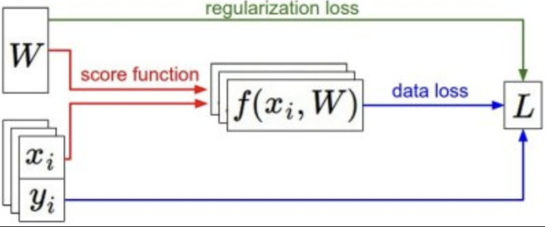
   • score function 将原始数据映射到标签。（线性）
   • loss function 衡量参数质量。（Softmax, SVM）data loss + regularization loss
   • optimization 寻找使得损失函数最小化的参数 W。
2. 后面将 线性映射 扩展到更复杂的神经网络，CNN，损失函数和优化过程不变。

2. Visualizing the loss function

1. W 高维可视化困难，生成随机权重矩阵 W，对应空间中的单个点。然后往某个方向走，记录 loss。
   假设随机方向 W1，loss 为 \(L(W + aW_1)\) a 的值作为 x 轴，loss 值作为 y 轴。损失函数表现为分段线性。
2. 考虑一个简单的数据集，包含三个一维的点。完整的 SVM 损失: 三条折线。
   x 轴为单个权重，y 轴为 loss。

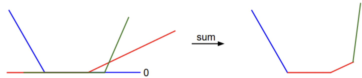
表现为凸函数，可以最小化。

但由于 max 操作，有拐点，该函数不可微分，因为拐点处梯度未定义。但是有 subgradient。

3. Optimization

损失函数：量化权重 W 的质量。

优化目标：找到使损失函数最小的 W。

1. Strategy #1: A first very bad idea solution: Random search
   随机生成 W，记录最小 loss 时的 W。ACC 15.5%
   核心思想：迭代。从一个随机的权重 W 开始，然后迭代改进。
   蒙眼走路，到达最低点。
   在 CIFAR-10 的示例中，山丘的维度为 30,730，因为 W 的维度为 10 x 3073。在山丘上的每个点，我们都会实现特定的损失（地形的高度）。
   Our strategy will be to start with random weights and iteratively refine them over time to get lower loss

2. Strategy #2: Random Local Search
   随机向一个方向走，如果是下坡，即损失更低，迈出一步。ACC 21.4%

3. Strategy #3: Following the Gradient
   计算下降最快的方向。即梯度最大，每个维度的偏导数： \(\frac{df(x)}{dx} = \lim_{h->0}\frac{f(x+h) - f{x}}{h}\)

4. Computing the gradient

两种，数值梯度 慢近似，但是简单。解析梯度 快准确，但是需要微积分。

1. Computing the gradient numerically with finite differences
   有限差分。用上文偏导公式求梯度，用 h 值逼近。数值梯度评估复杂度高。

def eval_numerical_gradient(f, x):
  """
  a naive implementation of numerical gradient of f at x
  - f should be a function that takes a single argument
  - x is the point (numpy array) to evaluate the gradient at
  """

  fx = f(x) # evaluate function value at original point
  grad = np.zeros(x.shape)
  h = 0.00001

  # iterate over all indexes in x
  it = np.nditer(x, flags=['multi_index'], op_flags=['readwrite'])
  while not it.finished:

    # evaluate function at x+h
    ix = it.multi_index
    old_value = x[ix]
    x[ix] = old_value + h # increment by h
    fxh = f(x) # evalute f(x + h)
    x[ix] = old_value # restore to previous value (very important!)

    # compute the partial derivative
    grad[ix] = (fxh - fx) / h # the slope
    it.iternext() # step to next dimension

  return grad

• 更新参数：沿梯度的负方向更新参数，因为希望损失函数减少。

• 步长：沿着该方向走多远，学习率。
• 小步长 持续，但缓慢。
• 大步长 变得快，但风险大。较大步长会升loss

# for step size 1.000000e-07 new loss: 2.135493
# for step size 1.000000e-06 new loss: 1.647802
# for step size 1.000000e-05 new loss: 2.844355
# for step size 1.000000e-04 new loss: 25.558142

1. Computing the gradient analytically with Calculus
   微积分。直接求梯度表达式。根据权重对损失函数微分。

5. Gradient Descent

1. 梯度下降：重复计算损失函数的梯度，然后评估梯度，更新参数的过程。
   在实践中，总是使用解析梯度，然后执行梯度检查，其中将其实现与数值梯度进行比较。

# Vanilla Gradient Descent

while True:
  weights_grad = evaluate_gradient(loss_fun, data, weights)
  weights += - step_size * weights_grad # perform parameter update

1. Mini-batch gradient descent.
   计算部分数据的梯度，然后更新参数。这样一轮可以更新很多次。
   因为训练样本间有相关性，少量可以代表整体。小批量计算出的梯度近似整体。
   通过计算 mini-batch 的梯度频繁更新参数，实现更快收敛。

# Vanilla Minibatch Gradient Descent

while True:
  data_batch = sample_training_data(data, 256) # sample 256 examples
  weights_grad = evaluate_gradient(loss_fun, data_batch, weights)
  weights += - step_size * weights_grad # perform parameter update

1. Stochastic Gradient Descent (SGD)
   极端情况：batch 很小。同 “Batch gradient descent”。
   batch 大小通常基于内存限制，或设置为 2 的幂：32，64. 因为许多向量化运算实现在其输入大小为 2 的幂时运算更快。

• 向前传递：计算 score，计算 loss，计算权重的梯度，更新参数 W。

总结

1. loss 量化了 W 的质量。optimazation：寻找使 loss 最小的参数 W。从随机权重开始，迭代。
2. 梯度下降：计算 loss 梯度，沿反方向更新参数 W。
3. 步长：学习率，必须恰到好处。
4. mini-batch：一轮参数更新多次，实现更快收敛。
5. SGD：迭代计算梯度并在循环中执行参数更新。
6. SVM 的 cost function 是分段线性，碗状凸函数。
7. 如何计算任意 loss 的梯度？反向传播？链式法则？